( ESNUG 513 Item 6 ) -------------------------------------------- [11/01/12]
Subject: Solido Brainiac explains how the Solido 6 sigma yield claims work
> I am wearing my engineer hat today, so I thought I'd point out some of
> the fundamental flaws in Solido's 6 sigma coverage claims...
>
> - Dr. Mehmet Cirit of Library Tech
> http://www.deepchip.com/items/0512-06.html
From: [ Trent McConaghy of Solido Design ]
Hi, John,
I appreciate the interest that Mehmet Cirit has demonstrated with respect to
Solido's High-Sigma Monte Carlo (HSMC) product. Mehmet made a number of
incorrect assumptions about Solido HSMC and also raised some points of
common confusion that I would like to address. I will start with the basic
blocks of high-sigma analysis and build upward:
- Modeling process variation at the device level
- Modeling process variation at the circuit level
- Modeling performance variation at the circuit level
- Monte Carlo (MC) sampling
- The high-sigma analysis problem
- Solido High-Sigma Monte Carlo (HSMC)
From this foundation, I will then address Mehmet's specific concerns.
Finally, I will compare high-sigma analysis techniques, for thoroughness.
MODELING PROCESS VARIATION AT THE DEVICE LEVEL
In modern PDKs supplied by foundries, each locally-varying process parameter
of each device is modeled as a distribution. On top of this, global process
variation is either modeled as a distribution, or as "corners" bounding a
distribution.
An example statistical model of device variation that is widely used,
accurate, and physically-based is the back propagation of variance (BPV)
model (Drennan and McAndrew 1999). The BPV model has one n-dimensional
distribution for each device (i.e. a transistor), and an n-dimensional
distribution for global variation. Each of the variables captures how the
underlying, physically independent process parameters change.
In the example below, the parameters are flatband voltage Vfb, mobility mu,
substrate dopant concentration Nsub, length offset deltaL, width offset
deltaW, short channel effect Vtl, narrow width effect Vtw, gate oxide
thickness tox, and source/drain sheet resistance rho_sh. More physical
parameters may be added.
 Variation of these physical process parameters leads directly to variation
(in silicon, and in simulation) of a device's electrical characteristics
like drain current Id, input voltage Vgs, transconductance gm, and output
conductance gd.
The random variables in these models may be normally distributed, log-
normally distributed, uniformly distributed, and so on. Furthermore,
random variables aren't always independent - they can be correlated.
MODELING PROCESS VARIATION AT THE CIRCUIT LEVEL
To model variation of process parameters at the circuit level, we have a
local variation distribution for every single device, plus a distribution
for global variation.
The figure below illustrates local variation on a simple Miller operational
transconductance amplifier (OTA). In the OTA, there are 64 local process
variables and 9 global process variables, for 73 process variables total.
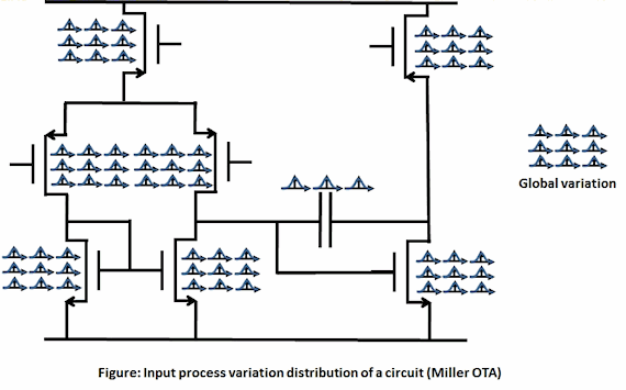 As a rule-of-thumb, on modern foundries' PDKs, we can expect at least 10
process variables per device, and perhaps 10 global process variables.
A 100-device circuit like a big opamp has 1,000 variables, and a 10,000
device circuit like a phase-locked loop (PLL) has 100,000 variables.
MODELING PERFORMANCE VARIATION AT THE CIRCUIT LEVEL
In circuits, the distributions of all physical local variations, and global
variations, map directly to variations in a circuit's performance
characteristics, such as gain, bandwidth, power, delay, etc. We want to
know the distribution of the circuit's performances.
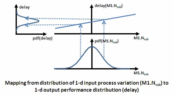
One distribution can map to another distribution via functions. As an
example, the fig below shows how a 1-d input process variable distribution
(the substrate doping concentration Nsub of transistor M1) is mapped to a
1-d output performance distribution (delay). In this example, the output
distribution is a shifted and scaled version of the input distribution, but
more nonlinear transformations may happen. Note that "pdf" is short for
"probability density function", and is just another label for
"distribution".
 The figure below generalizes this concept to a more general circuit setting,
where the input is a high-dimensional distribution describing process
variations, the mapping function is a SPICE circuit simulator (e.g. Spectre,
HSPICE, FineSim), and the output distribution describes performance
variations.
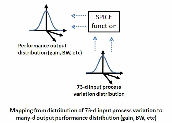 The output pdf has one dimension for each output performance, such as gain
and bandwidth (BW).
---- ---- ---- ---- ---- ---- ----
MONTE CARLO SAMPLING
Thanks to the statistical device models that are part of modern PDKs from
foundries like TSMC and GlobalFoundries, we have direct access to the
distributions of the *input* process variables. However, we do not have
direct access to the distributions of the *output* performances; mainly
because SPICE is a black-box function. It is these *output* distributions
that we care about - they tell us how the circuit is performing and what
the yield is.
Fortunately, we can apply the tried-and-true Monte Carlo (MC) sampling
method to learn about the output pdf and the mapping from input process
variables to output performance.
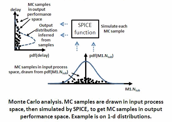 In MC sampling, samples (points) in *input* process variable space are drawn
from the *input* process variable distribution. Each sample (process point)
is simulated, and corresponding *output* performance values for each sample
are calculated. The figure above shows the flow of MC samples in *input*
process variation space, mapped by SPICE to MC samples in *output*
performance space.
---- ---- ---- ---- ---- ---- ----
THE HIGH-SIGMA ANALYSIS PROBLEM
The main goal in high-sigma analysis is to extract high-sigma tails of
circuit performances. For example, we may wish to find the 6-sigma "read"
current of a bitcell. (6 sigma is 1 failure in a billion.)
A simple way would be to draw 5 billion or so Monte Carlo samples (MC),
SPICE-simulate them, and look at the 5th-worst read current value. The
figure below illustrates.
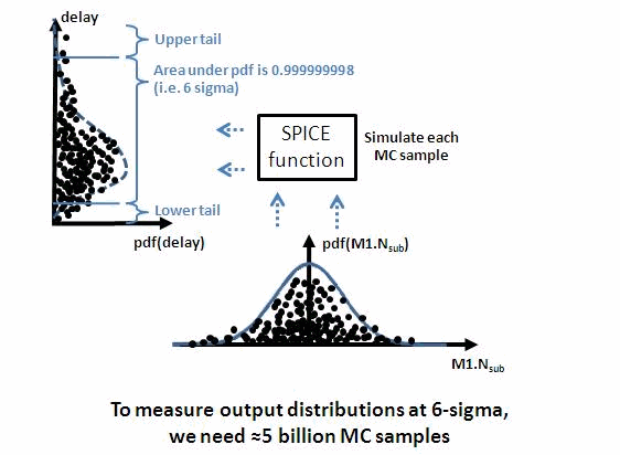 Of course, doing 5 billion sims is infeasible. With a 1 sec simulation
time, 5 billion simulations would take 159 years. We need a faster way.
Addressing this headache is important not only for bitcells, but also for
sense amps, digital standard cells, clock trees, medical devices, automotive
devices, and more - wherever failure is bad for the chip (e.g. standard
cells) or *catastrophic* to the wearer (e.g. medical).
---- ---- ---- ---- ---- ---- ----
SOLIDO HIGH-SIGMA MONTE CARLO (HSMC)
At Solido, we spent extensive effort investigating existing high-sigma
approaches, such as worst-case distances and importance sampling; none of
them had the required combination of speed, accuracy, scalability, and
verifiability. I'll go into more details on this later.
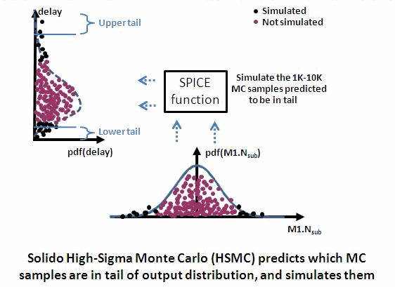
So, at Solido we ultimately invented the "High-Sigma Monte Carlo" (HSMC)
method, which we use in our product of the same name. The main idea of
the HSMC method is to draw all 5 billion MC samples from the *input*
process variable space, but simulate *only* the samples at the *tails*
of the *output* performance distribution. This is illustrated below.
 When the user runs Solido's HSMC tool, here is what it does automatically
"under the hood":
1. Draws (but doesn't simulate) 5 billion MC samples.
2. Chooses some initial samples, and simulates them. The samples are
chosen to be "well-spread" in the process variable space.
3. Data-mines the relation from *input* process variables to *output*
performance.
4. Rank-orders the 5 billion MC samples, with most extreme *output*
performance values first.
5. Simulates in that order, up to 1K-20K simulations. Periodically
re-orders using the most recent simulation results.
6. Constructs the tail of the *output* performance distribution, using
the simulated MC samples having the most extreme performance.
The figure below illustrates Solido HSMC behaviour over time, after the
first rank ordering. On the left, it has simulated the most extreme tail
samples. Then, it progressively fills the tail more deeply.
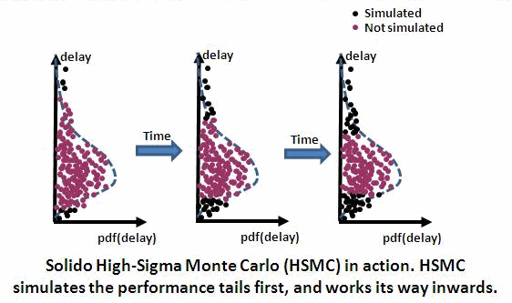 With a handful of quad-core machines, HSMC will find the performance tails
from 5 billion MC samples (6 sigma) for a bitcell in about 15 minutes.
---- ---- ---- ---- ---- ---- ----
A key attribute of Solido HSMC is its verifiability: we can tell if HSMC
performs poorly by using an output vs. sample convergence curve such as the
one in the figure below. In this example, HSMC is aiming to find the upper
tail of the bitcell's read current performance distribution, from 1.5
million MC samples generated.
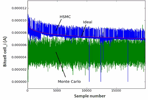 For the purposes of this example, we simulated all 1.5 M of the generated
samples to have ideal data. The "ideal" curve is computed by sorting the
1.5 M read current values; the first 20 K samples are plotted. We see that
it monotonically decreases, as expected of an ideal curve.
The "Monte Carlo" curve is the first 20 K simulations of MC sampling. As
expected, it has no trend because its samples were chosen randomly; its
output values distribute across the whole range. So of course, MC is very
slow at finding the worst-case values; we can only expect it to find all
worst-case values once it has performed all 1.5M simulations.
The HSMC curve has a general downward trend starting at the maximum value,
with some noise in its curve. The trend shows that Solido HSMC has captured
the general relation from process variables to output value. The noise
indicates that the HSMC model has some error, which is expected. The lower
the modeling error, the lower the noise, and the faster that HSMC finds
failures. The HSMC curve provides transparency into the behaviour of HSMC,
to understand how well HSMC is performing in finding failures. This is a
major part of the "verifiability" of HSMC: the user can view the curve to
tell if HSMC is working as expected. The clear trend shows that HSMC is
working correctly and is capturing the tail of the distribution.
---- ---- ---- ---- ---- ---- ----
MY RESPONSES TO MEHMET'S QUESTIONS
With this foundation, I'll now address Mehmet's specific questions.
> 1. Solido claims that by taking samples at the tails, they can cover
> as much terrain as if they did millions or billions of Monte Carlo
> SPICE simulations. Intrinsic in this claim is that the regions of
> design interest are the tails of the distributions.
>
> This is only partially true.
>
> If we are talking about a variable like threshold voltage, the bigger
> the increase, the bigger would be the delays. In such a case,
> sampling the tail make sense. However, circuits are very non-linear
> systems. For example, still talking about the delay, if you increase
> the width of a transistor, it will switch on faster. However, its
> driver will slow down because of the increase in the gate capacitance
> of the bigger transistors.
>
> In this case, best case delay will happen NOT at the tails, but closer
> to the center. Similarly for the worst case. Depending on the size
> and driver of each transistor, each can change the width up or down to
> have the worst total delay.
> Unfortunately, most of the variational parameters fall into this
> category. Depending on what you may call "failure" criteria, the
> region of interest varies, and when there are hundreds of variables,
> there is no way of guessing where the region of interest could be.
> Definitely it is not at the tails.
First, I would like to correct Mehmet's misunderstanding of what Solido HSMC
does. To be clear: HSMC finds the tails of the *performance* distribution.
It does not simply look at the tail values of the *process variables*.
Other than that, I completely agree with Mehmet. Yes, best/worst delay
(a performance) might not occur at the tail of process variables. And
that's ok! Yes, the region of interest can greatly vary, and the extreme
performance values could be anywhere in the process variable space. And
that's ok too! Solido HSMC is designed explicitly to identify the regions
of process variables that cause extreme performance values. It does this
using adaptive data mining, with feedback from SPICE. HSMC does this even
if there are 100's of process parameters. (It has even been applied to
problems with 10,000+ process parameters.)
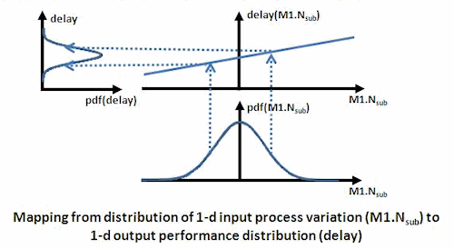 Let's illustrate Mehmet's concerns. The figure above had a single Gaussian-
distributed input process variable (M1.Nsub). It has a linear mapping to
the output performance (delay), and therefore the output performance is
Gaussian-distributed, too. In this scenario, we could simply pick extreme
values of M1.Nsub to get extreme values of delay.
Mehmet's concern is that this simple approach does not work for nonlinear
mappings, such as when "best case" is near nominal. I wholeheartedly agree
such a simple approach would not work. The figure below illustrates the
problem.
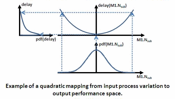 Taking extreme values of M1.Nsub would give maximum-extreme values of delay
(worst case). But to get minimum-extreme values of delay (best case), we
need samples near *nominal* values of M1.Nsub.
The figure below shows how Solido HSMC behaves in the scenario of quadratic
mapping.
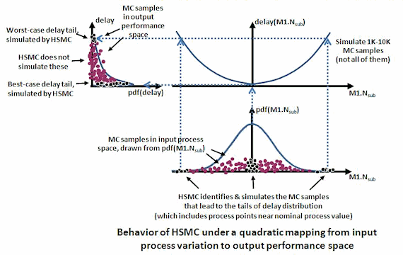 To get minimum-extreme samples of delay, HSMC simulates MC process points
near the nominal values of the M1.Nsub process distribution. And for
maximum-extreme delay, HSMC will simulate extreme M1.Nsub values. HSMC
will have figured out which samples to take via its data-mining to relate
M1.Nsub to delay.
---- ---- ---- ---- ---- ---- ----
> 2. If you have a priori knowledge of�the region of interest, then there
> is no need for Solido to do anything else. �There is no need to do
> simulation to find out your coverage. Just look it up from the
> Handbook of Mathematical Functions. I bought a copy at graduate
> school, it is still on my shelf.
If we had a priori knowledge of the region (or regions) of interest, then it
is correct that we might not need a high-sigma analysis tool. But as Mehmet
also pointed out, there can be 100's of process variables. We would need
to know the region for each of these 100's of variables. This is far from
trivial: we must possess an understanding of the intricate relation from the
complex device models and their statistical process parameters, to the
circuit's dynamics and the effect on the circuit performance. And of
course, that changes with each different circuit topology, each different
environmental condition, and each process node. The devices themselves
might even be dramatically different (FinFETs anyone?).
Managing this complex mapping under a wide range of scenarios is exactly
what SPICE simulators are designed to do. Solido HSMC leverages SPICE
simulators to adaptively data-mine and identify the region(s) of interest,
across a broad range of circuit topology, environmental conditions, and
process node settings.
We at Solido go out of our way for our tools to give back to the designer
whatever insight our tools might glean, for designer to add their own
insights and design knowledge in making decisions. For example, Solido HMSC
reports the impact of each process variable (or device) to the designer,
interactive plots of the distributions / tails, along with many other
visualizations.
---- ---- ---- ---- ---- ---- ----
> 3. It is a fallacy for Solido to claim that there is a random variable,
> ranging from minus infinity to plus infinity, controlling the length
> and width and various other parameters with some linear relationship.
I would like to correct Mehmet here also. Solido has never made claims that
random variables must exist ranging from minus infinity to plus infinity.
Nor has Solido ever made claims that device or circuit performances must be
a linear function of statistical variables. And we never would.
In fact, at Solido, we go out of our way to support whatever distribution
the device modeling folks come up with -- HSMC handles a wide range of
distributions. We go out of our way to support extremely nonlinear
mappings -- this is one of Solido's core competencies. It is not easy, and
requires state-of-the-art data mining. However, that is precisely one of
our core competencies. (I've been doing it since the late 90's, when I
worked on battlefield radar problems for national defense.)
---- ---- ---- ---- ---- ---- ----
> If you keep pushing this model towards the tails, you can easily get
> into a region where transistor length and width and other parameters
> may start assuming a non-physical character, like negative values, or
> push the device models into a region which may be contradictory, or
> the models may not extrapolate properly, or fail mathematically.
>
> What may happen at the tails are two fold:
>
> (a) such devices may not exist at all, and
> (b) interpolated device models may be not realistic
> and may not interpolate.
>
> 4. These distribution models are only reliable for relatively small
> variations around the center.
> Unfortunately, that region is not specified in the models.
> Any Solido variation assumptions outside that region are suspect.
This is a description of issues pointed out *and solved* by device modeling
experts back in the 1990s. Yes, some statistical models are terrible. But
thoughtfully-designed modern ones are very good. Good yield estimates
affect the bottom line in high volume circuits, which gives incentive to
develop good statistical models. A good example of a sane, physically-based
model is the Back-propagation-of-variance model (BPV) of Drennan and
McAndrew (IEDM 2009), which I described earlier. More recently, researchers
have been calibrating the models better for 6 sigma, such as the work by
Mizutani, Kumar and Hiramoto (IEDM 2011) as my previous Deepchip post on
6-sigma analysis discussed in http://www.deepchip.com/items/0505-06.html.
---- ---- ---- ---- ---- ---- ----
> Finally let me point out that Solido's 6 sigmas could be very deceptive
> especially when you talk about local random variations. For example, if
> you qualify a 6 transistor RAM cell to have 1PPM�failure under random
> variations, and if you have 1 million of them on a chip, that chip will
> always have one failure, for sure. You need much higher level 1PPT
> reliability from low level components to have 1PPM reliability at the
> chip level.
Note that Mehmet's argument that 1 PPM failure rate means you always have
one failure for every million is not statistically accurate, just as when I
toss a coin two times, it will not always have one head.
Beyond this technical correction, I interpret Mehmet's core concern as
follows, and I agree with it: if we have 1 failure in a million, we need
more than 1 million samples to have a sufficiently accurate answer (i.e.
to have tight confidence intervals, or to have a low variance statistical
estimate). Just as I wouldn't declare "90% yield" with confidence based
on seeing 1 failure from 10 MC samples.
However, the solution to this concern is trivial, and is exactly what
Solido HSMC users do in practice: they generate 5-20x the number of MC
samples compared to the number of failures they expect. For example, if
they expect about 1 failure in a billion, they generate 5-10 billion MC
samples.
REVIEW OF HIGH-SIGMA ANALYSIS APPROACHES
Many high-sigma analysis approaches exist - I will review them here. These
approaches can be measured according to four factors: speed, accuracy,
scalability and verifiability.
- Speed: Degree of reduction in simulations required compared to the
traditional Monte Carlo method.
- Accuracy: Compare to the accuracy given by 5 billion MC samples.
- Scalability: Ability to handle a large number of input process
variables. A 6-transistor bitcell with 10 local process variables
per device has 60 *input* process variables. A sense amp might
have about 150. Larger circuits can easily have 1,000 or 10,000
or more *input* process variables.
- Verifiability. When running the approach in a design scenario,
can the user tell if the approach works or fails? For example,
when SPICE fails, the user can tell because KCL or KVL are violated.
It is extremely important to be able to identify and avoid scenarios
where the approach fails, because that can mean over-estimating
yield or performance.
The chart below compares the high-sigma approaches on multiple key factors.
Approaches to High-Sigma Estimation (MC = Monte Carlo)
|
Standard MC |
Solido High-Sigma MC |
Importance Sampling |
Extrapolation |
Worse Case Distance |
| Simulation Reduction Factor |
1 X |
1 Million X |
1 Million X |
1 Million X |
1 Million X if linear. Worse if quadratic. |
| Accuracy |
YES.
Draws samples from actual distr. until enough tail samples. |
YES.
Draws samples from actual distr., simulates tail samples. |
NO.
Distorts away from the actual distr. towards tails. |
NO.
From MC samples, extrapolates to tails. |
NO.
Assumes linear or quadratic, Assumes 1 failure region. |
| Scalability |
YES.
Unlimited process variables |
YES.
1000+ process variables |
NO.
10-20 process variables |
YES.
Unlimited process variables |
OK / NO.
# process variables = # simulations - 1 (if linear). Worse if quadratic. |
| Verifiability |
YES.
Simple, transparent behavior |
YES.
Transparent convergence (akin to SPICE KCL/KVL) |
NO.
Cannot tell when inaccurate |
NO.
Cannot tell when inaccurate |
NO.
Cannot tell when inaccurate |
Below I have more detailed data on each approach.
- Traditional MC. It scales to an unlimited number of process variables,
since MC accuracy is only dependent on the number of samples. It is
also familiar to designers, simple, and easy to trust. However,
simulating 5 billion samples is infeasibly slow for production designs.
- Solido High-Sigma Monte Carlo (HSMC). HSMC is accurate because it uses
SPICE, it uses MC samples, and it's tolerant to imperfect ordering
because its tail uses only extreme-valued simulations. HSMC scales to
a large number of process variables because it uses MC samples and MC
is scalable, and its data mining is scalable, having roots in "big data"
regression on millions of input variables. Finally, it is verifiable
via monitoring its convergence curve, as described earlier.
- Importance Sampling (IS). The idea here is to distort the sampling
distribution with the hope that it will cause more samples to be near
the performance tail. The figure below illustrates.
 One challenge is *how* to distort the distribution: get it wrong and
we will miss the most probable regions of failure, leading to over-
optimistic yield estimates. To do it reliably, we must treat it as
a global optimization problem, which to solve reliably is exponentially
expensive in the number of process variables. For example, the
computational complexity is 10^60 with 60 *input* process variables
(6 devices). Even worse, we have no way of telling when Importance
Sampling has failed. Also, since IS approaches typically assume a
single region of failure, they are inaccurate with >1 failure regions.
Finally, we have found that designers are often uncomfortable to learn
that the sampling distribution gets distorted, as Importance Sampling
does.
- MC with extrapolation. Draw 10K-100K MC samples, simulate them, and
then extrapolate the performance distribution to the high-sigma tails.
This of course suffers the classic problem of extrapolation: inaccuracy.
We will never know whether the distribution bends, or drops off, or
whatever, farther out. This can lead to vast over-estimation or
under-estimation of yield.
- Worst-Case Distance (WCD). One variant of WCD is to do sensitivity
analysis, construct a linear model from process variables to
performance, then estimate yield. Of course, assuming "linear" has
major inaccuracy on nonlinear mappings, even simple quadratic mappings
like described above.
Nonlinear WCD methods exist too; they are typically quadratic.
Unfortunately, these approaches scale much worse with the number of
process variables. For example, 1000 process variables needs
1000 * (1000 - 1) / 2 = about 500,000 simulations
and is still restricted to quadratic models. All WCD approaches
assume just a single region of failure, which means they over-estimate
yield when there are >1 failure regions.
Regarding verifiability: because the linear model or quadratic model is
treated as "the" model of performance, we will never know whether the actual
mapping has higher-order interactions or other nonlinear components, which
could lead to major error in yield estimation. For example, we have seen
sharp dropoffs in the minimum-extreme value of read current in a bitcell,
and a linear or quadratic model would miss this.
CONCLUSION
I would like to thank Mehmet for his interest in HSMC, and his enthusiasm in
trying to identify issues. I hope that I have helped to illuminate what
high-sigma analysis is about, explained what Solido HSMC does, addressed
Mehmet's concerns, and shown how it relates to other high-sigma analysis
techniques.
Solido HSMC is already part of TSMC's Custom Design Flow (Wiretap 100728)
and in production use by IDM's and fabs for mem, std cell and analog design.
Here's a case study from an HSMC production user in ESNUG 492 #10.
- Trent McConaghy
Solido Design Vancouver, Canada
Join
Index
Next->Item
|
|


 One challenge is *how* to distort the distribution: get it wrong and
we will miss the most probable regions of failure, leading to over-
optimistic yield estimates. To do it reliably, we must treat it as
a global optimization problem, which to solve reliably is exponentially
expensive in the number of process variables. For example, the
computational complexity is 10^60 with 60 *input* process variables
(6 devices). Even worse, we have no way of telling when Importance
Sampling has failed. Also, since IS approaches typically assume a
single region of failure, they are inaccurate with >1 failure regions.
Finally, we have found that designers are often uncomfortable to learn
that the sampling distribution gets distorted, as Importance Sampling
does.
- MC with extrapolation. Draw 10K-100K MC samples, simulate them, and
then extrapolate the performance distribution to the high-sigma tails.
This of course suffers the classic problem of extrapolation: inaccuracy.
We will never know whether the distribution bends, or drops off, or
whatever, farther out. This can lead to vast over-estimation or
under-estimation of yield.
- Worst-Case Distance (WCD). One variant of WCD is to do sensitivity
analysis, construct a linear model from process variables to
performance, then estimate yield. Of course, assuming "linear" has
major inaccuracy on nonlinear mappings, even simple quadratic mappings
like described above.
Nonlinear WCD methods exist too; they are typically quadratic.
Unfortunately, these approaches scale much worse with the number of
process variables. For example, 1000 process variables needs
1000 * (1000 - 1) / 2 = about 500,000 simulations
and is still restricted to quadratic models. All WCD approaches
assume just a single region of failure, which means they over-estimate
yield when there are >1 failure regions.
Regarding verifiability: because the linear model or quadratic model is
treated as "the" model of performance, we will never know whether the actual
mapping has higher-order interactions or other nonlinear components, which
could lead to major error in yield estimation. For example, we have seen
sharp dropoffs in the minimum-extreme value of read current in a bitcell,
and a linear or quadratic model would miss this.
CONCLUSION
I would like to thank Mehmet for his interest in HSMC, and his enthusiasm in
trying to identify issues. I hope that I have helped to illuminate what
high-sigma analysis is about, explained what Solido HSMC does, addressed
Mehmet's concerns, and shown how it relates to other high-sigma analysis
techniques.
Solido HSMC is already part of TSMC's Custom Design Flow (Wiretap 100728)
and in production use by IDM's and fabs for mem, std cell and analog design.
Here's a case study from an HSMC production user in ESNUG 492 #10.
- Trent McConaghy
Solido Design Vancouver, Canada
Join
Index
Next->Item

